Complete Data Structures Guide: 7 Core Data Structures with Python Implementation

From Beginner to Expert: Master Core Data Structures and Their Applications

Data Structure

1. Core Data Structures Overview

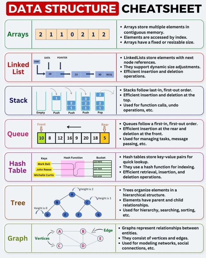
Let's first understand these seven fundamental data structures from a macro perspective.

1. Array

• Core Concept: Arrays store elements of the same type in contiguous memory space. Imagine numbered storage lockers, each the same size, adjacent to each other.
• Key Characteristics:
  • Fast Access: Can directly locate any element through index, time complexity is $O(1)$.
  • Fixed Size: Usually need to specify size when creating, not easily expandable. (Dynamic arrays like Vector or ArrayList solve this problem, but have performance overhead during expansion).
  • Slow Insert/Delete: Inserting or deleting elements in the middle of an array requires moving all subsequent elements, time complexity is $O(n)$.
• Use Cases: Scenarios that require frequent data reading with fewer insert/delete operations. For example, storing a set of fixed configuration items, serving as underlying implementation for other data structures (like stacks and queues).

2. Linked List

• Core Concept: Elements in a linked list (called "nodes") are stored non-contiguously in memory. Each node contains data and a pointer (reference) to the next node.
• Key Characteristics:
  • Dynamic Size: Can easily add or remove nodes, very flexible memory usage.
  • Efficient Insert/Delete: Only need to change adjacent node pointers, time complexity is $O(1)$ (if the target node is known).
  • Slow Access: Finding an element must start from the head node and traverse sequentially, time complexity is $O(n)$.
• Use Cases: Scenarios requiring frequent insert and delete operations. For example, implementing task queues, music player playlists, operating system memory management.

3. Stack

• Core Concept: A stack is a linear data structure that follows Last-In, First-Out (LIFO) principle. Imagine a stack of plates - you always put plates on top and take them from the top.
• Key Characteristics:
  • Only perform insert (Push) and delete (Pop) operations at the top.
  • Operations are very efficient, all $O(1)$.
• Use Cases:
  • Function Call Stack: Programs push function information onto the stack when calling functions, and pop when returning.
  • Undo/Redo operations.
  • Browser history (forward/backward).
  • Bracket matching validation.

4. Queue

• Core Concept: A queue is a linear data structure that follows First-In, First-Out (FIFO) principle. Like queuing for tickets - first come, first served.
• Key Characteristics:
  • Insert (Enqueue) at the rear, delete (Dequeue) at the front.
  • Operations are very efficient, all $O(1)$.
• Use Cases:
  • Task Scheduling: Managing pending tasks, like printer task queues.
  • Message Passing: Asynchronously passing messages between different system modules.
  • Breadth-First Search (BFS) algorithm.

5. Hash Table

• Core Concept: Hash tables use a hash function to map "keys" to storage locations ("buckets"), enabling fast access to key-value pairs.
• Key Characteristics:
  • Extremely fast lookup, insert, and delete: In ideal cases, time complexity approaches $O(1)$.
  • May experience hash collisions (different keys mapping to the same location), requiring collision resolution mechanisms (like chaining, open addressing).
• Use Cases: Almost everywhere! Whenever you need to quickly store and retrieve information through a unique identifier, hash tables should be your first consideration.
  • Database indexing.
  • Caching systems.
  • Dictionary/Map implementations in programming languages.

6. Tree

• Core Concept: A tree is a hierarchical non-linear data structure composed of nodes and edges connecting nodes, with clear parent-child relationships. The topmost node is the root, and each node (except root) has only one parent.
• Key Characteristics:
  • Hierarchical Relationships: Perfect for representing data with hierarchical structure.
  • Efficient Search: In specific types of trees (like binary search trees, B-trees), search, insert, delete operations are highly efficient, usually $O(\\log n)$.
• Use Cases:
  • File Systems: Directory and file organization structure.
  • HTML DOM: Web page structure is a tree.
  • Database Indexing (e.g., B+ trees).
  • Organizational charts.

7. Graph

• Core Concept: Graphs consist of vertices and edges connecting vertices, representing complex relationships between entities. Unlike trees, nodes in graphs can have arbitrary connections, even forming cycles.
• Key Characteristics:
  • Flexibility: Can simulate any network structure.
  • Edges can have direction (directed graph) or weight (weighted graph).
• Use Cases:
  • Social Networks: Users are vertices, friendships are edges.
  • Map Navigation: Locations are vertices, roads are edges, distances are weights.
  • Computer Networks: Devices are vertices, network connections are edges.
  • Recommendation systems.

2. Scenario Selection: Which One Should I Use?

When facing a specific problem, how to choose the most suitable data structure? Here's a simple decision flow:

When your requirement is...	Consider First	Reason
Fast access to elements by index, with fixed data size	Array	Unmatched $O(1)$ read speed.
Frequent insertion and deletion, don't care about random access speed	Linked List	Extremely efficient $O(1)$ insert/delete operations.
Managing "last-in, first-out" tasks or data	Stack	Perfect fit for LIFO scenarios like function calls, undo operations.
Processing tasks in order, ensuring fairness	Queue	FIFO principle ensures processing order, like task scheduling, message queues.
Fast storage, lookup, or deletion by unique key	Hash Table	Near $O(1)$ average performance, first choice for performance optimization.
Representing hierarchical relationships, parent-child relationships, or ordered data sets	Tree	Suitable for organizational structures, file systems, binary search trees provide $O(\\log n)$ operation efficiency.
Representing complex many-to-many relationships, network connections	Graph	Natural modeling approach for social networks, map path planning problems.

A Comprehensive Example:

Suppose you're developing a shopping cart feature for an e-commerce website.

• Product list in shopping cart: Both array or linked list work. If product count is small and fixed, array is simpler; if users frequently add/remove products, linked list is more flexible.
• Quickly find product info by product ID in cart: Use hash table (Product ID -> Product Object), enabling $O(1)$ location for quantity/price updates.
• Product categories (e.g., Electronics -> Phones -> iPhone): This is clearly hierarchical structure, should use tree.
• Recommend "people who bought this also bought...": Build a graph where products are vertices, user co-purchase behavior creates edges connecting them.

Python Data Structures Implementation

1. Array -> Python's list

In Python, we typically use the list type as a dynamic array. It automatically handles memory allocation and expansion, very convenient.

Core Concept: Python's list is a dynamic array, meaning it can grow or shrink as needed. Its elements are stored contiguously in memory (making indexed access very fast).

# 1. Creation and initialization
# Create a list containing integers
my_array = [2, 1, 1, 0, 2, 1, 2]
print(f"Initial list: {my_array}")

# 2. Access elements (O(1) - very fast)
# Access the third element by index (starting from 0)
element = my_array[2]
print(f"Element at index 2: {element}")

# 3. Modify elements (O(1))
my_array[3] = 99
print(f"Modified list: {my_array}")

# 4. Add elements
# a) Add at end (append) - average O(1)
my_array.append(5)
print(f"After appending 5: {my_array}")

# b) Insert at specific position (insert) - O(n)
# Insert number 88 at index 1
my_array.insert(1, 88)
print(f"After inserting 88 at index 1: {my_array}") # Note: all elements after 88 moved backward

# 5. Delete elements
# a) Remove last element (pop) - O(1)
last_element = my_array.pop()
print(f"After removing last element ({last_element}): {my_array}")

# b) Remove element at specific position (pop) - O(n)
removed_element = my_array.pop(1) # Remove element at index 1
print(f"After removing element at index 1 ({removed_element}): {my_array}")

# 6. Get list length (O(1))
print(f"Current list length: {len(my_array)}")

Key Points:

• Advantages: Reading/writing through index my_array[i] is very fast.
• Disadvantages: insert or pop at the beginning or middle of the list is slow because it requires moving many elements.

---

2. Linked List

Python doesn't have a built-in linked list type, but we can easily create one using class.

Core Concept: Composed of nodes (Node), each node contains data and a reference (next) to the next node.

# First define the node class
class Node:
    def __init__(self, data):
        self.data = data  # Data stored in the node
        self.next = None  # Reference to next node, default None

# Then define the linked list class
class LinkedList:
    def __init__(self):
        self.head = None  # Head node of the list, default None

    # Add new node at the end of the list
    def append(self, data):
        new_node = Node(data)
        if not self.head:  # If the list is empty
            self.head = new_node
            return
        # Otherwise, traverse to the end of the list
        last_node = self.head
        while last_node.next:
            last_node = last_node.next
        last_node.next = new_node

    # Print all node data in the list
    def display(self):
        elements = []
        current_node = self.head
        while current_node:
            elements.append(current_node.data)
            current_node = current_node.next
        print(" -> ".join(map(str, elements)))

# Using the linked list
my_linked_list = LinkedList()
my_linked_list.append(10)
my_linked_list.append(20)
my_linked_list.append(30)

print("Linked list content:")
my_linked_list.display() # Output: 10 -> 20 -> 30

Key Points:

• Insert and delete operations (if you know the previous node of the target) are very fast, only need to modify next references, time complexity $O(1)$.
• Finding a node requires traversing from head, time complexity $O(n)$.

---

3. Stack - LIFO

In Python, you can directly use list to simulate a stack, because append() and pop() operations at the end of the list are both $O(1)$.

# Using list to implement stack
my_stack = []

# Push
my_stack.append(1)
my_stack.append(2)
my_stack.append(3)
print(f"After pushing: {my_stack}") # Output: [1, 2, 3]

# Pop
top_element = my_stack.pop()
print(f"Popped top element: {top_element}") # Output: 3
print(f"After popping: {my_stack}") # Output: [1, 2]

# Peek at top element
peek_element = my_stack[-1]
print(f"Current top element: {peek_element}") # Output: 2

Better Choice: Use collections.deque. Although list works, deque (double-ended queue) is optimized for adding and removing elements at both ends, making it ideal for implementing stacks and queues.

---

4. Queue - FIFO

Using list to implement a queue is inefficient because removing elements from the beginning (pop(0)) is an $O(n)$ operation. The correct approach is to use collections.deque.

Core Concept: deque provides the popleft() method, enabling $O(1)$ complexity for removing front elements.

from collections import deque

# Create queue using deque
my_queue = deque()

# Enqueue
my_queue.append(10)
my_queue.append(8)
my_queue.append(12)
print(f"After enqueuing: {my_queue}") # Output: deque([10, 8, 12])

# Dequeue
front_element = my_queue.popleft() # O(1) operation, very efficient!
print(f"Dequeued front element: {front_element}") # Output: 10
print(f"After dequeuing: {my_queue}") # Output: deque([8, 12])

# Peek at front element
if my_queue:
    print(f"Current front element: {my_queue[0]}") # Output: 8

Key Point: When implementing queues, always prefer collections.deque.

---

5. Hash Table -> Python's dict

Python's dictionary (dict) is a powerful and highly optimized hash table implementation.

Core Concept: Stores key-value pairs (key: value) and quickly locates the value corresponding to a key through hash functions.

# 1. Creation and initialization
my_hash_table = {
    "Mark Bell": "123-4567",
    "John Reese": "321-7654",
    "Michelle Curtis": "456-1234"
}
print(f"Hash table: {my_hash_table}")

# 2. Access elements (average O(1))
# Get value by key
phone_number = my_hash_table["John Reese"]
print(f"John Reese's phone: {phone_number}")

# 3. Add or modify elements (average O(1))
# Add new entry
my_hash_table["Harold Finch"] = "999-9999"
# Modify existing entry
my_hash_table["Mark Bell"] = "111-2222"
print(f"After modification: {my_hash_table}")

# 4. Delete elements (average O(1))
del my_hash_table["Michelle Curtis"]
print(f"After deletion: {my_hash_table}")

# 5. Check if key exists (average O(1))
if "Harold Finch" in my_hash_table:
    print("Harold Finch is in the hash table.")

Key Point: dict is one of the most important data structures in Python. When you need to establish mapping relationships or fast lookups, it's almost always the best choice.

---

6. Tree

Like linked lists, trees also need to be defined using class. Here's a simple binary tree node definition.

class TreeNode:
    def __init__(self, key):
        self.key = key      # Node value
        self.left = None    # Left child node
        self.right = None   # Right child node

# Manually build a tree (corresponding to the example in the image)
#     A
#    / \
#   B   C
#  / \ / \
# D  E F  G

# Create nodes
root = TreeNode('A')
root.left = TreeNode('B')
root.right = TreeNode('C')
root.left.left = TreeNode('D')
root.left.right = TreeNode('E')
root.right.left = TreeNode('F')
root.right.right = TreeNode('G')

# Tree traversal (example: inorder traversal - left, root, right)
def inorder_traversal(node):
    if node:
        inorder_traversal(node.left)
        print(node.key, end=' ')
        inorder_traversal(node.right)

print("Inorder traversal result:")
inorder_traversal(root) # Output: D B E A F C G

Key Point: The power of trees lies in their recursive structure. Many operations (like search, traversal) can be completed with concise recursive functions.

---

7. Graph

In Python, the most common way to represent graphs is using adjacency lists, typically implemented with a dictionary where each key is a vertex and the value is a list of vertices adjacent to that vertex.

# Implement adjacency list using dictionary and lists
# Corresponding to the example in the image
graph = {
    'A': ['B', 'C'],
    'B': ['A', 'D', 'E'],
    'C': ['A', 'D'],
    'D': ['B', 'C', 'E'],
    'E': ['B', 'D']
}

# Print graph structure
for vertex, neighbors in graph.items():
    print(f"Vertex {vertex} connects to: {neighbors}")

# Find all neighbors of a vertex (O(1))
print(f"\nNeighbors of vertex B: {graph['B']}")

# Simple graph traversal algorithm: Breadth-First Search (BFS)
def bfs(graph, start_node):
    visited = set()     # Record visited nodes
    queue = deque([start_node]) # Start from the starting node
    visited.add(start_node)
    
    while queue:
        vertex = queue.popleft()
        print(vertex, end=' ')
        
        for neighbor in graph[vertex]:
            if neighbor not in visited:
                visited.add(neighbor)
                queue.append(neighbor)

print("\nBFS traversal starting from vertex A:")
bfs(graph, 'A') # Possible output: A B C D E

Key Point: Adjacency list representation is very space-efficient for sparse graphs (where the number of edges is much smaller than the square of the number of vertices) and can quickly find all neighbors of a vertex.

---