Introduction to LLM Architectures
From Llama 3 to Kimi K2: A Visual Guide to Modern LLM Architectures
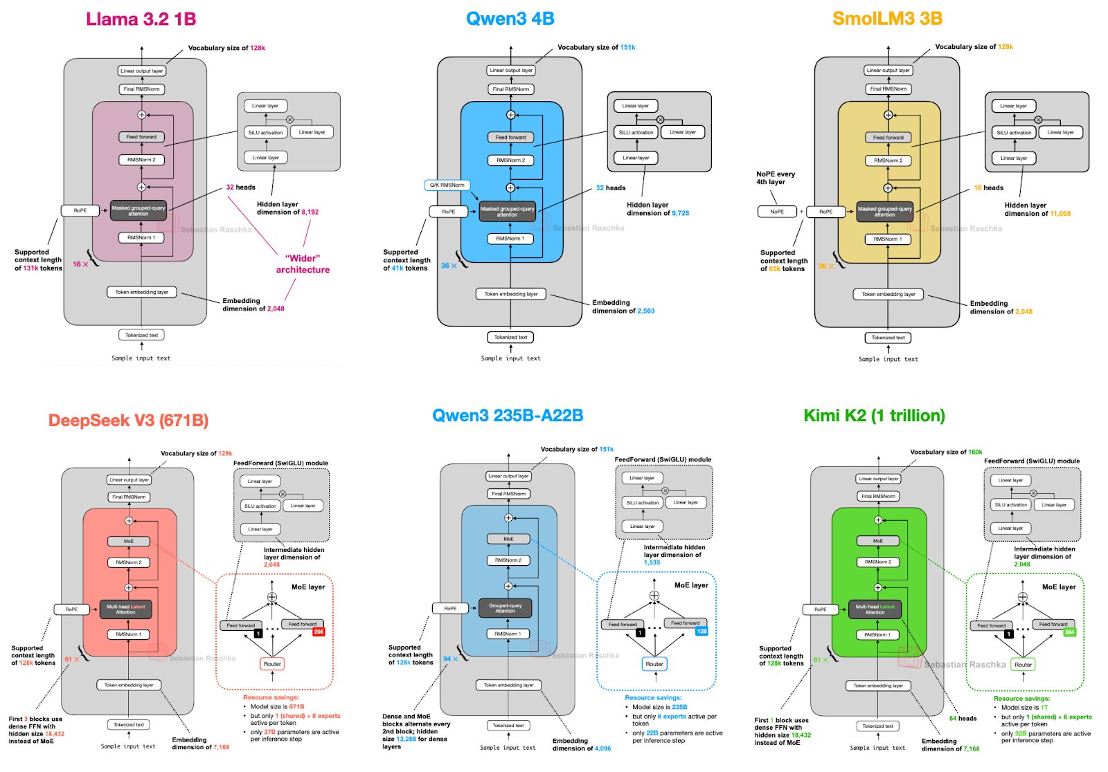
Recently, a clear comparison image of the architectures of six mainstream large language models (LLMs) has been widely circulated in the tech community. From lightweight models with tens of billions of parameters to massive models with trillions, this image provides us with an excellent window to observe how the most cutting-edge LLMs are designed and built today.
For many friends interested in AI, the "black box" inside the model always seems mysterious. This article will use this image as a blueprint to analyze the architectural features of these models one by one, explain the key technical concepts, and help you not only "watch the excitement" but also "understand the principles".
Core Technical Concepts: Building Your Knowledge Framework
Before delving into each model, let's first understand several core technical terms that appear repeatedly in the image. Once you understand them, you will grasp the key to reading LLM architectures.
- Vocabulary Size: This is like the "dictionary" size of the model. It determines how many different words or "tokens" the model can directly understand and generate. The larger the vocabulary, the stronger the model's ability to handle multiple languages or specialized terminology.
- Supported Context Length: This is the length of text the model can "remember" and process at one time, usually measured in tokens. For example, a context length of 128k means the model can read and analyze a novel with hundreds of thousands of words and perform Q&A or creation on this basis without "forgetting" the beginning. This is a key indicator of the model's ability to handle long texts.
- Embedding Dimension: Inside the model, text cannot be directly computed and needs to be converted into numerical vectors first. This process is called "embedding". The embedding dimension is the length of this vector. Generally, the higher the dimension, the richer and more detailed the semantic information the vector can carry about a word.
- Hidden Layer Dimension: This is the width of the "thinking" space inside the model. In each layer of the network, the input data is transformed into a higher-dimensional space for processing. The larger this dimension, the stronger the model's feature extraction and expression ability, but it also requires more computing resources.
- Attention Heads: This is the key component of the "attention mechanism" in LLMs. If the attention mechanism allows the model to focus on different parts of the text, then multi-head attention enables the model to focus on the text from multiple perspectives at the same time. For example, one head may focus on grammatical structure, another on semantic associations. The more heads, the richer the perspectives the model can analyze the text from.
- FeedForward (SwiGLU) & MoE:
- FeedForward Network (FFN): This is another core component in the Transformer architecture, responsible for non-linear processing of information extracted by the attention mechanism, enhancing the model's expressive ability.
- SwiGLU: A highly efficient variant of FFN. You can think of it as a smarter "gate" mechanism that better controls information flow, making model training more stable and effective. As seen in the image, it has become a standard configuration for modern LLMs.
- Mixture of Experts (MoE): This is a "smart" strategy to cope with the explosive growth of model scale. Imagine you don't need to consult all the experts in a company for every problem, just find the most relevant ones. MoE follows this principle. It divides the huge model into multiple "expert" subnetworks, and only a small number of the most relevant experts are activated for each data processing. This allows the model to maintain relatively low actual computational cost even with a huge number of parameters.
Six Major Model Architectures: From Compact to Massive
Now, with these concepts in mind, let's start our journey through model architectures. We divide the models into two groups: classic dense models and cutting-edge Mixture of Experts (MoE) models.
Group 1: Classic Dense Models—Solid Foundation
The feature of this type of model is that all parameters are activated for each computation.
Llama 3.2 1B & SmolLM3 3B:
- Commonality: These two can be regarded as representatives of small-scale models. They both use relatively traditional dense architectures, with standard vocabulary sizes (128k) and medium-to-lower context lengths (8k-16k).
- Llama 3.2 1B's "Wider" Architecture: The special feature of Llama 3.2 is its "wider" design. Compared to making the network "deeper", it chooses to increase the hidden layer dimension (4,192), making it far surpass models of the same parameter scale. The idea is that a wider network may be more efficient in feature extraction and processing.
- SmolLM3 3B's NoPE: It explicitly marks "NoPE", meaning no positional encoding. This usually means it uses more advanced methods like RoPE (Rotary Positional Encoding) to handle token position information, which is already mainstream in modern LLMs.
Qwen3 4B:
- Ultra-long Context: Its biggest highlight is the support for a context length of up to 128k, which is quite amazing among models with tens of billions of parameters, showing its ambition in long text processing.
- Balanced Design: Its various parameters (embedding dimension, hidden layer dimension) are relatively balanced, without special "widening" like Llama 3.2, representing a more classic balanced design approach.
Group 2: Mixture of Experts (MoE) Models—The Road to Trillion Parameters
As model parameters break through the trillion mark, MoE has become the "standard answer". Its core advantage is to use lower computational cost in exchange for huge model capacity and performance.
DeepSeek V3 (671B):
- Extreme MoE: DeepSeek V3 is a massive model with 671 billion parameters. It has 160 experts, but only 9 are activated each time. This means that only a small part of the parameters are actually involved in computation, greatly saving inference cost.
- Shared Experts: It also introduces the concept of "shared experts", which are used by all computations to handle some common knowledge, while other experts handle more specialized information.
Qwen3 235B-A22B:
- "Active" Parameters: The "A22B" in the model name is key information, meaning that although the total parameters are 2.35 trillion, only 220 billion are actually active.
- Efficient Routing: It has 64 experts, with 4 activated each time. This design ensures model performance while also achieving efficient computation routing, a typical application of MoE architecture.
Kimi K2 (1 trillion):
- Trillion-parameter "Giant": Kimi K2 is currently at the peak of parameter scale, reaching an astonishing 1 trillion. It also uses MoE architecture to manage such a huge number of parameters.
- Fine-grained Routing: With 128 experts and 2 activated each time, this "needle in a haystack" routing strategy can accurately match the most suitable knowledge unit for specific tasks in a massive knowledge base (experts). This allows Kimi K2 to maintain strong capabilities while keeping inference costs controllable.
Core Technical Concept Flowchart Descriptions:
- Embedding Flow:
- Single-head Attention Mechanism Flow:
- Multi-head Attention Mechanism Flow:
- Mixture of Experts (MoE) Simplified Flow:
Key Component Diagram Descriptions of Model Architecture:
Transformer Block Simplified Structure:
Now, let's combine these diagram descriptions to understand the key knowledge points in more detail:
Detailed Explanation of Core Technical Concepts and Diagram Understanding
Embedding:
Flowchart Description:
- Input:
Original text (e.g.: "I love you") - Arrow:
-> through embedding layer -> - Output:
Numerical vectors (e.g.: [0.2, -0.5, 0.8, ...], [0.1, 0.3, -0.9, ...], [0.7, -0.1, 0.4, ...])(each word corresponds to a vector)
- Input:
Explanation: The embedding layer converts human-readable words into dense vectors that machines can understand and compute. These vectors are learned during training, so that words with similar meanings are closer in vector space.
Single-head Attention Mechanism:
Flowchart Description:
- Input:
Query (Q), Key (K), Value (V)(all are linear transformations of the input text) - Step 1:
Calculate attention weights: similarity(Q, K) -> weights(e.g., dot product then Softmax normalization) - Step 2:
Weighted sum Value: weights × V -> attention output
- Input:
Explanation: The core idea of the attention mechanism is to allow the model to "focus" on the relevance between words in the input sequence when processing a word. Query represents the "query", Key represents the "key being queried", and Value represents the "value being queried". By calculating the similarity between Query and Key, it can determine which Keys (and corresponding Values) should be "emphasized".
Multi-head Attention Mechanism:
Flowchart Description:
- Input:
Query (Q), Key (K), Value (V) - Parallel Processing (multiple "heads"):
Head 1: Q1, K1, V1 -> attention output 1Head 2: Q2, K2, V2 -> attention output 2...Head N: QN, KN, VN -> attention output N
- Concatenation:
Concatenate(attention output 1, attention output 2, ..., attention output N) -> concatenated vector - Linear Transformation:
concatenated vector × weight matrix -> multi-head attention output
- Input:
Explanation: Multi-head attention allows the model to learn different attention patterns from different subspaces at the same time. Each "head" focuses on different aspects of the input, and finally combines these different attention points to provide richer contextual information.
Mixture of Experts (MoE):
Flowchart Description:
- Input:
Input data - Router Network:
Input data -> calculate scores for each expert -> determine which experts to activate - Parallel Processing (selected experts):
Expert 1 (selected): input data -> output of expert 1Expert 2 (selected): input data -> output of expert 2...
- Combination Mechanism:
output of expert 1, output of expert 2, ... -> weighted sum or more complex combination -> MoE output
- Input:
Explanation: The key to MoE is its sparsity. Not all parameters participate in every computation, but a routing mechanism determines which "expert" subnetworks should process the current input. This allows the model to maintain relatively high computational efficiency while having a huge number of parameters.
Detailed Explanation and Diagram Understanding of Transformer Block Structure
**Transformer Block**:

* **Flowchart Description**:
    * **Input**: `Output from previous layer or original input`
    * **Residual Connection 1**: `Input -> split -> one path directly to adder`
    * **Multi-head Self-attention**: `Another path -> multi-head self-attention layer -> output`
    * **Add & LayerNorm 1**: `Residual Connection 1 + multi-head self-attention output -> LayerNorm -> output 1`
    * **Residual Connection 2**: `Output 1 -> split -> one path directly to adder`
    * **Feedforward Neural Network**: `Another path -> feedforward neural network -> output`
    * **Add & LayerNorm 2**: `Residual Connection 2 + feedforward neural network output -> LayerNorm -> output 2`
    * **Output**: `Output 2 -> next layer`

* **Explanation**:
The Transformer Block is the basic building block of modern LLMs.
It consists of a multi-head self-attention mechanism and a feedforward neural network,
and introduces residual connections and layer normalization to improve the training process.

    * **Self-attention**: The model can focus on the relationships between words at different positions in the input sequence.
    * **Feedforward Neural Network**: Performs independent non-linear transformations on the representation of each position, enhancing the model's expressive ability.
    * **Residual Connection**: Helps alleviate the vanishing gradient problem in deep network training, allowing information to skip certain layers directly.
    * **Layer Normalization**: Speeds up training and improves the generalization ability of the model.
Summary and Insights: The Future Trend of LLM Architectures
Through this image, we can clearly see several important industry trends:
- MoE is the only way to larger models: When model parameters exceed the trillion level, MoE becomes almost the only choice. It perfectly balances the contradiction between model "capacity" and "computational cost".
- Context length continues to increase: From the initial thousands of tokens to today's 128k or even longer, the ability of LLMs to handle long texts is developing rapidly, unlocking more application scenarios such as long document analysis and full-book Q&A.
- Efficient components become standard: Functions like SwiGLU and methods like RoPE have become the "standard configuration" of modern LLM architectures due to their superior performance and stability.
- Diversity in architectural design: Even under similar scales, model designers are still exploring different possibilities, such as the "widening" strategy of Llama 3.2. This diversity drives the entire field forward.